Satellite Link Budget for A Nonlinear Bent-Pipe Transponder

In 1973, J.C. Fuenzalida and colleagues published a study pertaining to nonlinear characteristics of High Power Amplifiers (HPAs). The study showed that nonlinear HPA not only amplifies the uplink carriers (identified by the satellite front-end receiver Input Back Off, or IBO) but also produces unwanted harmonic carriers in the proximity of the downlink primary carriers (identified by the spacecraft transmitter Output Back Off, or OBO) in the transponder. These unwanted harmonic carriers are the Inter-Modulation (IM) products of the primary carriers. These IM products not only rub power from the primary carriers, but also cause interference to the primary carriers. The interfering component is the IM power and its amplitude is related to the nonlinearity of the HPA. The study showed that the higher the nonlinearity, the higher the IM products and the lower the Carrier-to-Intermodulation product ratio (C/IM).

The purpose of this study is to use these variables (e.g., IBO, OBO and IM) plus two other spacecraft variables, Saturate Flux Density (SFO) and the saturated Effective Isotropic Radiated Power (EIRPsaturated) from the nonlinear characteristics of the transponder HPA to formulate a simple satellite link budget.

A satellite link budget provides a possible solution for the earth station and the spacecraft transmitter power (e.g., EIRP) in a particular Earth-to-space-to-Earth communication link. The traditional textbook expression for an uplink carrier-to-thermal noise ratio (C/Nup) could be expressed as [2]:

C/Nup = EIRPe – Lpu + G/Ts – k – 10Log(BW) (1a)

where:

EIRPe = the uplink earth station effective isotropically-radiated power (dBW);

Lpu = the path loss, at the operating frequency, between the earth station and the spacecraft (dB);

G/Ts = the spacecraft receiving antenna gain-to-system noise temperature (dB/k);

k = Boltzmamn’s constant (Joules/K), –228.6 dBW/HzK;

BW = the emission (or carrier) bandwidth (Hz)

Converting the above equation to spacecraft transponder elements — in particular, the Saturated Flux-Density (SFD) at the spacecraft receive antenna toward the transmitting earth-station location and the IBO of the spacecraft HPA — the resulting equation could be expressed as:

C/Nup = SFD + IBO + G/Ts + 10Log(lλ2/4π) – k – 10Log(BW) (1b)

where λ is the uplink frequency wavelength (m). Similarly, using the spacecraft saturated EIRP toward the desired receiving earth station location (e.g., EIRPsaturated) and the OBO, the downlink carrier-to-thermal noise ratio (C/Ndown) could be expressed as:

C/Ndown = EIRPsaturated + OBO – Lpd + G/Te – k – 10Log(BW) (2)

where:

Lpd = the downlink path loss at the downlink operating frequency between the spacecraft and the receiving earth station location (dB);

G/Te = the earth station receiving antenna gain-to-system noise temperature (dB)

IBO, OBO, C/IM and Transponder Linerarity

As indicated by the first two terms in C/Nup (equation 1b) or C/Ndown (equation 2), the spacecraft power amplifier may not always be operating at saturation. In other words, the deviation from saturation is being identified by the input back off (IBO), in equation 1b, and the output back off (OBO), in equation 2.

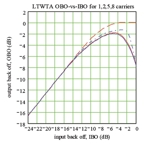
According to Fuenzalida’s published study, the relationship between IBO and OBO of a typical spacecraft HPA (e.g., TWTA, LTWTA or SSPA) is not linear but rather nonlinear because it reflects the behavior of the spacecraft nonlinear HPA within each transponder. The following figure illustrates the nonlinear OBO-vs-IBO behavior of a LTWTA. The two dashed curves represent one (dash red) and two (dash blue) carriers. And the two solid curves represent five (solid red) and eight (solid blue) carriers operating within the transponder.

The curves, within the figures, highlight the behavior of OBO as a function of IBO for various numbers of Equal-Power/Equal-Bandwidth (EPEB) carriers sharing the transponder. The curves also highlight the linearity of the amplifiers. Linearity is illustrated by the straightness of the curves. For example, the LTWT amplifier has a linear transfer characteristics for output-back-off less than about –7 dB.

Fuenzalida’s study further demonstrated that, due to the nonlinear characteristics of the transponder HPA, the HPA not only amplifies the uplink carriers (primary carriers) but also produces unwanted harmonic carriers in the proximity of the primary carriers in the transponder. These unwanted harmonic carriers are the IM products of the primary carriers. These IM products not only rub power from the primary carriers but also cause interference to the primary carriers. The interfering component is the intermodulation power and its amplitude is related to the nonlinearity of the HPA. Fuenzalida et al. [1] showed that, the higher the primary carriers in the transponder, the higher the intermodulation products and the lower the carrier-to-intermodulation product ratio (C/IM). This is illustrated in the following figure for the LTWT amplifier in Figure-1

SFD and Attenuator Setting

In a simple-frequency-changing transponder (e.g., bent-pipe transponder), there is a telecommand control to set the amplification or power gain of the transponder by the uplink telecommand signal from the Telemetry, Tracking and Command (TT&C) station. The purpose of the power gain setting, or Attenuator Setting (ATTS), is to control the SFD level to saturate the spacecraft power amplifier. At the required SFD level, the transponder produces the maximum output power (i.e., saturated output power or EIRPsaturated). In a nutshell, the attenuator setting controls the uplink sensitivity of the transponder. In other words, the attenuator setting allows the uplink earth station to saturate the transponder at various SFD levels. Specifically, the SFD at any spacecraft-receiving antenna G/T contour could be determined by the following equation:

SFDo = SFDr + (G/Tr – G/To) + (ATTSo – ATTSr) (3)

where:

SFDo = the operating SFD level (dBW/m2);

SFDr = the reference SFD level (dBW/m2); for example, the minimum SFD

at the spacecraft receiving antenna peak G/T (e.g., at beam peak);

G/Tr = the reference G/T level (dB/k); for example, the spacecraft beam peak G/T;

G/To = the operating G/T level (dB/k);

ATTSo = the operating attenuator setting (dB) for the operating G/T;

ATTSr = the reference attenuator setting (dB)

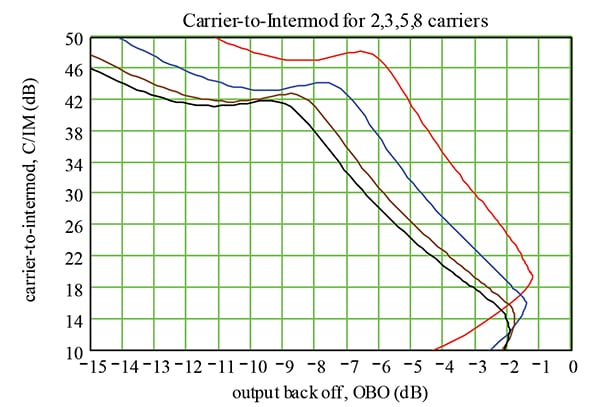
Figure-2 Carrier-to-intermodulation product

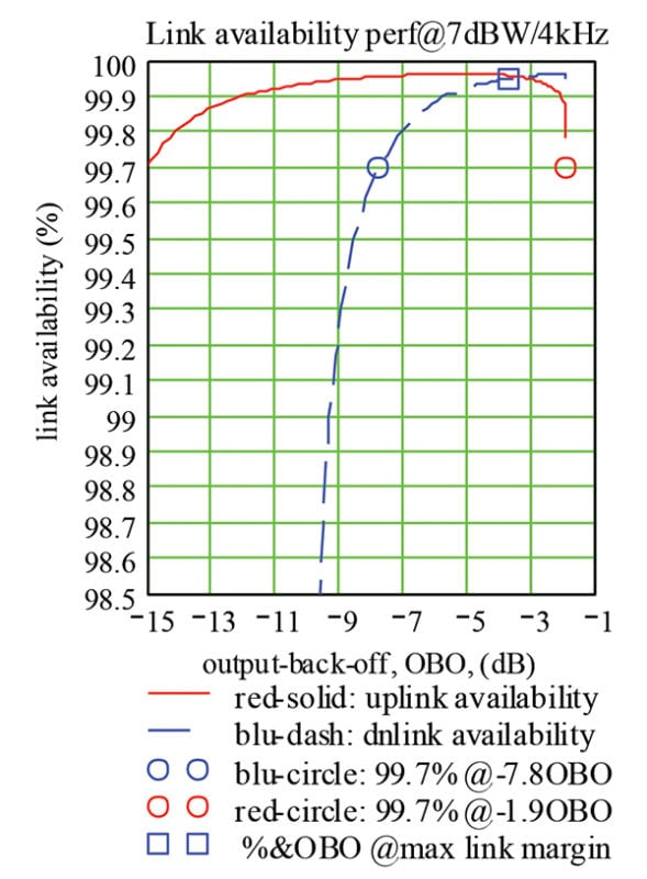
Figure-4 GSO satellite link availability

Satellite Link Budget

Using a satellite link model as suggested by J.H. Cook for an earth station-to-space station-to-earth station bent-pipe transmission, the carrier-to-noise plus intermodulation-interference ratio at the receiving earth station output could be expressed as:

C/(N+IM) = [(C/Nu)-1 + (C/Nd)-1 + (C/IM)-1]-1 (3)

where:

C/Nu = the uplink carrier-to-thermal noise ratio (dB);

C/Nd = the downlink carrier-to-thermal noise ratio (dB);

C/IM = the carrier-to-intermod ratio (dB);

Yet, in a complex geostationary-satellite-orbit network, there are other internal and external impairments. Internal impairments are caused by network elements such as earth station and spacecraft antenna polarizers, which create the orthogonal signals. The external impairments are caused by the adjacent satellite networks, for example, adjacent-satellite downlink EIRP density.

To complete an overall/full picture analysis of a satellite link, J.H. Cook also showed that these impairments could be included in the link budget in the following way:

C/(N+I+IM) = [ (C/Nu)-1 + (C/Nd)-1 + (C/IM)-1 + (C/Xu)-1 + (C/Xd)-1 + (C/Iu)-1 + (C/Id)-1 ]-1 (4)

where:

C/Xu = the uplink carrier-to-cochannel orthogonal signal ratio (dB);

C/Xd = the downlink carrier-to-cochannel orthogonal signal ratio (dB);

C/Iu = the uplink carrier-to-adjacent satellite interference (dB);

C/Id = the downlink carrier-to-adjacent satellite interference (dB)

In a congested geostationary satellite orbital arc, there could be two close-by-adjacent satellites, one to the east and the other to the west, along the orbital arc. There are two sets of corresponding C/Is. This is the net received signal power at the receiving earth station demodulator input and it determines the satellite link performance.

Using the information contained in Figure-1 (i.e., IBO and OBO) and Figure-2 (i.e., C/IM) and assuming an SFD and EIRPsaturated value for a typical FCC domestic satellite, Figure-3 plots the link budgets for an external downlink interference of 7 dBW/4kHz and an uplink interference of –14 dBW/4kHz. The consecutive link budgets are based on successive pairing of IBO/OBO from near saturation to -15 dB below transponder saturation (see Figure 1). At each successive step, the IBO value is used to determine the uplink carrier-to-thermal noise ratio (C/Nup, the red-solid curve in Figure-3), the OBO value is used to determine the downlink carrier-to-thermal noise ratio (C/Ndn, the blue-solid curve in Figure-3) and the C/IM plus the external downlink interference of 7 dBW/4kHz are used to determine the carrier-to-interference ratio (C/(N+I+IM)).

The resulting link budget is plotted in Figure-3. This figure provides a visual heuristic search of possible solutions for a sub-optimum or a preferred link budget. The figure shows that the operating OBO could be as low as –10.55 dB. At this operating point, the earth station received signal level (i.e., C/(N+I+IM)) is equal to the demodulator threshold. In other words, the link margin is approximately equal to zero (i.e., C/(N+I+IM) – demodulator threshold = 0.0). Therefore, for clear-sky operations, the OBO operating point could be as low as –10.55 dB and as high as –1.9 dB.

One of the preferred link budgets — through the heuristic search — could be the maximum link margin case. This is identified by the black-circle in the figure. At this transponder operating point, the operating margin is equal to 5.44 dB (13.55 – 8.11 = 5.44). This is the maximum link margin that the satellite network could have in this example link budget.

The link margin varies from 0 dB (at OBO = -10.55) to 5.44 dB (at OBO = -3.74) and to 2.84 dB (at OBO = -1.9). These positive link margins could be used to compensate for rain attenuation in either the uplink or downlink. The duration of rain-attenuation time outage could be determined from ITU-R propagation model. Using these positive link margins, Figure-4 plots the satellite link availability for the uplink and downlink. This figure provides a visual heuristic search of a required link availability; for example, the figure identifies the operating OBO for 99.7 percent availability and for the maximum link margin. VS

Harold Ng
Prior to his retirement, Harold Ng worked for the FCC, NTIA, PanAmSat, ICO and SES Americom with focus in domestic and international technical and regulatory standards in satellite communication service.