Make Sense of Nonlinear Distortion Part 2: Predicting and minimizing distortion

In Part 1, we viewed nonlinear distortion as a level-dependent shift in modulation, amplitude and phase. Next, we use that technique to predict system performance and avoid the pitfall of nonlinear distortion memory.

Predicting Nonlinear Behavior

If the system is memoryless, then the response to any waveform can be predicted with numerical simulation. There is no closed-form general solution, but the computation algorithm is straightforward:

1. Find or measure the Amplitude-to-Amplitude (AM-AM) and Amplitude-to-Phase (AM-PM) curves that are valid for the center frequency and across the bandwidth of interest. Remember, the algorithm only works if these curves do not change, or change only slightly, over that bandwidth.
2. Determine a simulation time step. It must be no less than the Nyquist sampling rate for the highest frequency component in the modulation spectrum.
3. Generate a sample modulation waveform. This could be a two-tone signal, multi-tones, Quadrature Phase Shift Keying (QPSK) modulation, multiple carriers, noise, a noise power ratio (NPR) waveform, or any limited-bandwidth signals of interest. It needs to be long enough to cover the lowest frequency components in the modulation. In order to avoid windowing artifacts, it helps to make the sample length as long as possible and the sampling rate higher, perhaps four times the highest component.
4. Step through the modulation waveform in time. For each step, calculate the instantaneous power and phase of the modulation signal.
5. Use the power value to look up the values of the AM-AM and AM-PM curve. Use interpolation to avoid quantization artifacts.
6. Record the resultant output power as your instantaneous output power. Add the resultant phase to the input waveform phase to get your instantaneous output phase.
7. Repeat steps 4 through 6 through the entire input waveform.

You now have an output waveform in the form of a complex time-domain modulation of the original arbitrary carrier. If you plot it and overlay it on the input waveform, you can observe phenomena such as clipping and compression. But in most cases, you will want to pass it through a fast fourier transform (FFT) so you can see the resultant spectrum which will reveal intermodulation products, sideband regrowth, NPR, and other useful metrics. You can find variations on this algorithm in system simulators from AWR Corporation, Agilent Technologies, and others. At SatProf, we wrote our own code, with versions for Matlab, Excel Visual for Basic Applications (VBA) macros, and Flash ActionScript for integration into online interactive training materials.

Nonlinear transfer curves can be measured in many ways, such as swept-power vector network analyzers (VNA), pulsed VNA, and specrtal-null pulse (SNP). In all of these, the characterization requires considerable laboratory craft and care.

Once you have characterized your device or system, you can use the simulation analysis to predict any performance metric, such as sideband regrowth, two-tone intermodulation distortion (IMD), allowed cell rate (ACR) and NPR. You can cascade or parallel nonlinear systems too, and predict linearizer performance, effects of imbalance in phase-combined amplifiers, and other system metrics. For a given general shape of the nonlinear transfer curves, you can even propose rational relationships for hard-to-measure specifications like NPR against easy-to-measure metrics like two-tone IMD.

Memoryless Systems

Experience dictates that distortion memory rarely improves performance. For example, we have seen a situation in which the measured NPR of a solid-state power amplifier (SSPA) was much worse than predicted from the AM-AM/AM-PM curves, although its two-tone IMD performance matched the prediction. Troubleshooting revealed a resonance in a bias circuit, which introduced a “ringing” response in the operating point of the gallium arsenide field-effect transistor (GaAs FET). Damping that resonance improved NPR performance. The only obvious example of distortion memory in a device helping performance is within a linearizer that not only matches an amplifier’s AM-AM/AM-PM curves but also adaptively matches its distortion memory behavior. Such linearizers are commonly used in wireless base station amplifiers, which have around 100 MHz bandwidth, but rarely in satellite uplinks, which need at least 500 MHz bandwidth.

What Causes Distortion Memory?

Distortion memory becomes appreciable when:

a) there is some parameter within the system that varies with the power level and affects gain and phase response; and

b) that parameter has a long response time compared to the time scale of the complex modulation of the signal set.

One example is thermal effects in a field-effect transistor (FET) or bipolar device. In all devices, some more than others, gain varies with temperature. For example, in a GaAs FET, small signal gain drops at higher temperatures by about 0.007 dB per degree C, depending on bias scheme. At higher powers, the heat dissipated in a FET is a function of the signal power level. And the thermal time constant of the GaAs structure can be quite long, meaning microseconds (μsec). Figure 1 shows an amplifier being pulsed with a CW signal. If the pulse amplitude takes the amplifier output only into low level, the output amplitude instantly follows the input envelope at both the leading and trailing edges of the pulse. But if the input level is increased enough that the leading edge brings the output to near the 1dB compression point, the level quickly drops as the device heats and its gain falls over a few μsec, eventually reaching equilibrium. When the signal is removed, the device begins to cool and again the output envelope displays a transient response. Clearly, if one were to stimulate the amplifier with a two-tone signal, the time-averaged IMD response would depend on the relationship between the tone spacing, the pulse repetition rate, and the thermal time constant.

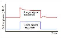
Figure 1: Pulse response of an amplifier with thermal
distortion memory

Bias resonances are another common cause of distortion memory. Bias voltage and current obviously affect gain, but large signal conditions can cause, for example, changes in drain or gate current. If the bias network does not preset a low impedance at the modulation frequencies, this change in current will cause a voltage change which will, in turn, affect the gain. Bias networks, however, must present high impedances at the carrier frequency. In between, there can be spurious responses, such as a resonance of a bias choke with a bypass capacitor as shown in Figure 2. If the amplifier is stimulated with an envelope that varies at a similar rate to that resonance, the amplifier’s gain and phase response could be quite different than its continuous wave (CW) response.

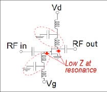
Figure 2: Bias resonances that may cause distortion memory

A third source of distortion memory is simply narrowband small-signal response of the radio frequency (RF) chain. Imagine, for example, placing a 20-MHz-wide band pass filter in front of an amplifier that has significant, but memoryless, nonlinearity. Then simulate this system with a 20-MHz-wide QPSK signal. At the wider spacing, the filter’s gain and phase response alters the input amplitude and relative phases of the spectral components of the QPSK signal, which changes how the modulated signal maps into the AM-AM/AM-PM curves over time. In other words, the group delay and amplitude variation across the linear filter’s bandpass has the effect of causing a nonlinear distortion memory in the filter-amplifier system.

There are several ways to determine empirically if your system has distortion memory that could be causing unexpected degradation in nonlinear performance.

The most obvious, but generally least accurate, way is to pulse the system with a short CW signal. If the output envelope measured over time, for example with a wideband diode detector on an oscilloscope, does not match the input envelope, then there is distortion memory.

A better way is to use a two-tone IMD test and vary the spacing of the tones. If there is no distortion memory, the carrier-to-interface ratio (C/I) will be independent of the tone spacing, and the third-order products should remain at a constant level as the tones separate. Substantial variations suggest distortion memory. A significant difference between the upper and lower frequency products also suggests distortion memory.

Some Tips and Cautions:

• Make sure your two signal generators are not generating intermodulation in each other’s output amplifiers. Use isolators, a high-isolation combiner, and/or large-value attenuators to suppress the signal from one generator from reaching the other.
• Make sure the gain in your measurement system from generator to system under test is very flat across; at least three times the maximum tone spacing at which you will be testing.
• Test with a maximum tone spacing equal to the widest total bandwidth of the signal set that your system is specified to operate with. For example, if you are testing a Ku-band satellite uplink HPA, you may be required to meet an NPR specification with a notched noise signal with 500 MHz bandwidth. To fully emulate the time of change of this stimulus signal, a two-tone signal spacing should be swept up to 500 MHz.
• Test with a minimum tone spacing that will catch either the slowest distortion memory effect you are looking for, such as a thermal effect, or represents the lowest frequency component of the signal set that your system is designed to pass.
• If you observe a high-pass or low-pass effect at narrow spacings, the distortion memory is likely due to thermal or similar effects.
• If you observe a rapid change in IMD response around a narrow frequency range, such as is illustrated in Figure 3, the distortion memory is likely due to a bias circuit resonance.
• You should test with a range of power levels. However, the distortion memory effect does not necessarily reduce with signal level, even though the IMD level itself reduces.

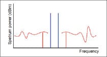
Figure 3: Searching for distortion memory effect with swept-spacing tones

Conclusion

Classic rules of thumb for predicting nonlinear performance do not work well close to compression. Satellite uplink high-power amplifiers are often amenable to characterization by AM-AM/AM-PM curves and accurate simulation based on complex modulation. Measured performance will be worse than predicted if the system has distortion memory, but distortion memory can be diagnosed using a swept-spacing, two-tone intermodulation test. That’s a worthwhile check for any large-signal system, even without simulation.